
Eight heads in ten flips do not prove a coin is biased. Nor does a run of twenty rolls without a six prove anything is wrong with a die. Probability simulations repeat the chance experiment and compare the outcomes with what a mathematical model predicts.
A game science lab puts a sharper question to each game: what should happen, how often, and under which rules? Coin tosses, dice games, prize spinners, card draws and player strategies can all be tested. A few memorable wins or losses tell little about the underlying odds.

Probability simulations at a glance
| Chance event | Theoretical probability | What to simulate |
|---|---|---|
| Heads on one fair coin flip | 1/2 = 50% | Heads versus tails |
| A seven from two fair six-sided dice | 6/36 = 1/6 ≈ 16.67% | Sum of both dice |
| A twelve from two fair six-sided dice | 1/36 ≈ 2.78% | Sum of both dice |
| Exactly two heads in three fair coin flips | 3/8 = 37.5% | Number of heads per three-flip trial |
| One chosen sector of a four-sector equal spinner | 1/4 = 25% | Sector reached by the pointer |
| Winning by switching in the standard Monty Hall game | 2/3 ≈ 66.67% | Switch versus stay strategy |
These are mathematical benchmarks, not guaranteed results for a fixed run. Even a correct simulation will fluctuate around them.
What is a probability simulation?
A probability simulation repeats a model of a random experiment. One trial produces an outcome, such as heads, a dice sum or a card. An event selects one or more outcomes: “the dice total is seven” covers six distinct pairs. The sample space is the full set of possible outcomes.
Theoretical probability follows from the rules. If every outcome in the sample space is equally likely, divide the number of favourable outcomes by the total. Experimental probability, or relative frequency, uses the counts observed across repeated trials:
Estimated P(event) = number of successful trials / total number of trials
Probabilities run from 0 (impossible under the model) to 1 (certain), or from 0% to 100%. If an event occurs 70 times in 200 trials, its observed frequency is 0.35. That alone does not establish a true probability of exactly 35%.
Coins, dice, counters, cards and spinners work for physical trials. A computer can imitate their rules with a random-number generator and repeat a trial thousands of times. A wrong model just delivers the wrong results faster.
How to design a trustworthy chance experiment
- State one precise question. “What fraction of two-dice rolls total seven?” is testable. “Are dice lucky?” is not.
- Specify the random mechanism. Record the number of coins or dice, spinner-sector weights, deck composition and whether drawn items are replaced.
- Define a full trial. For three flips, one trial means flipping three times and recording the number of heads. It does not mean counting every flip as a separate three-flip experiment.
- List or model the possible results. Build a sample-space grid, tree diagram or table of outcome probabilities before comparing data.
- Run a planned number of trials. Compare a short run of 10, a medium run of 100 and a larger run of 1,000 using the same rules.
- Record counts and proportions. Keep a frequency table, a bar chart or a line graph of running relative frequency. Mark the theoretical probability separately.
- Check the assumptions. Does the next event depend on the previous one? Is the device fair? Does a player change strategy after an outcome?
Changing the rules partway through makes the results incomparable. Keep separate datasets for each version. When testing two strategies, specify identical game conditions and record the number of trials for each.
Dice simulation: why seven appears more often than twelve
Two fair six-sided dice produce 36 equally likely ordered pairs. Each die has six faces, but the sums are not equally probable. Seven has six pairs: (1,6), (2,5), (3,4), (4,3), (5,2) and (6,1). Only (6,6) gives twelve.
| Sum | Ways to make each sum | Probability of each sum |
|---|---|---|
| 2 or 12 | 1 | 1/36 ≈ 2.78% |
| 3 or 11 | 2 | 2/36 ≈ 5.56% |
| 4 or 10 | 3 | 3/36 ≈ 8.33% |
| 5 or 9 | 4 | 4/36 ≈ 11.11% |
| 6 or 8 | 5 | 5/36 ≈ 13.89% |
| 7 | 6 | 6/36 ≈ 16.67% |
Tally the sum from each pair of dice. Over many trials, seven should appear more often than twelve, though a short run can reverse that order. Compare the bars with the exact 36-pair sample space before blaming the dice for a surprising chart.
The question changes if the game scores the difference between dice, counts doubles or adds three dice. Each requires its own event definition. A four-sided die (d4) and a twenty-sided die (d20) do not share the sample space of two d6 dice.
Coin flips: independence, streaks and compound events
Three fair coin flips give eight equally likely sequences: HHH, HHT, HTH, HTT, THH, THT, TTH and TTT. Exactly two heads occur in HHT, HTH and THH, giving 3/8, or 37.5%. At least two heads also includes HHH, giving 4/8, or 50%. The two questions need different success counters.
The count of heads follows a binomial distribution when the number of flips is fixed, flips are independent and each has the same chance of heads. A coin with a 70% chance of heads has a different distribution from a fair coin.
Five heads in a row can feel like a warning that tails is next. It is not. With an unchanged fair coin and independent flips, the next head still has probability 1/2. The belief that a losing or winning streak must reverse is the gambler’s fallacy. Recording next-flip results after many streaks makes the error visible.
Weighted spinners, mystery bags and card draws
A four-sector spinner with equal sectors assigns 25% to each. If red covers half the wheel, with blue and green taking one quarter apiece, P(red) = 1/2 and P(blue) = P(green) = 1/4. The total is 1. For a random-integer model using 1–8, assign 1–4 to red, 5–6 to blue, 7–8 to green. Using numbers 1–3 with one number per colour would accidentally make all colours equally likely.
Consider a mystery bag with three red counters and two blue. If the first draw goes back into the bag, the chance of drawing red twice is (3/5) × (3/5) = 9/25, or 36%. This is sampling with replacement: the draws are independent. Without replacement, four counters remain before the second draw, so the chance is (3/5) × (2/4) = 3/10, or 30%. Those draws are dependent.
A standard 52-card deck contains four suits and thirteen ranks. Drawing an ace, putting it back and drawing again is not the same experiment as dealing two cards without replacement. Shuffling between games does not restore a card after a draw within a game.
Is a game fair? Winning probability is only half the answer
A one-in-six win rate does not tell you whether a game is fair. Under an expected value definition of fairness, the average net score per play is zero over the long run. Neither a 50% win rate nor a zero score for every player is required.
Take a two-dice game. A seven wins +5 points; any other sum loses −1 point. Since seven appears with probability 1/6, the expected net score is:
E(points) = (1/6 × 5) + (5/6 × −1) = 0
That is a zero-expected-value game with fair dice. If the prize falls to +4 points, its expectation changes to:
E(points) = (1/6 × 4) + (5/6 × −1) = −1/6 point per play
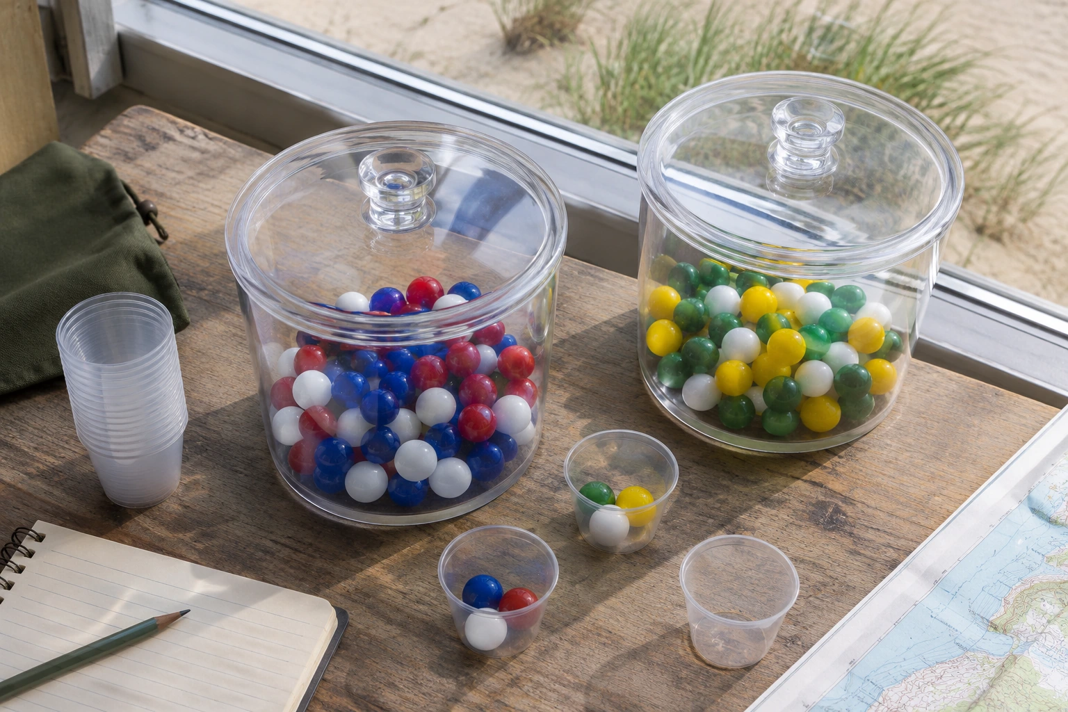
The organiser now gains about 0.167 points per play on average. Winners still exist; a short run can leave a player ahead. Expected value describes the long-run balance, not the next result. The game’s variance matters as well. Two games with the same expected value can have very different losses and streaks.
Points or counters keep a school gala or classroom fairness test separate from real-money gambling. If prizes run out, players have different skills or the rules shift, those factors must be represented in the model.
Monte Carlo simulation: thousands of virtual games
Monte Carlo simulation draws many random trials from an explicit model to estimate its outcomes. It handles multi-stage games, complex card combinations and strategies that are awkward to calculate by hand. For two dice, the procedure is simple:
Set wins = 0
Repeat 10,000 times:
    Roll die A uniformly from 1 to 6
    Roll die B independently from 1 to 6
    If die A + die B = 7:
        Add 1 to wins
Estimated chance of seven = wins / 10,000
The exact chance of seven is 1/6. A result from 10,000 simulated rolls will normally be close, not identical. If points matter, record the net score for each round and calculate its average as well as the win rate. For competing strategies, simulate the same rules under each one.
Digital simulations commonly use pseudorandom numbers. A fixed random seed reproduces a sequence for debugging or classroom comparisons. Running the same seed again repeats the old sample, rather than supplying an independent one. Another seed supplies a new run, but neither establishes the fairness of real dice, coins or commercial games.
How many trials are enough?
With 100 trials, the pattern may still be noisy. At 1,000, the proportion is usually steadier. Increasing the sample helps estimate a correctly specified model; no sample size guarantees an exact theoretical percentage.
The law of large numbers concerns the way a running mean or relative frequency approaches its expected value over many trials under suitable assumptions. A running line can drift away from theory before returning towards it. Absolute differences in counts need not shrink; compare proportions instead.
For independent win/loss trials with fixed probability p, the approximate standard error of the observed proportion is sqrt(p × (1 − p) / n), where n is the trial count. At p = 0.5, it is around 5 percentage points for 100 trials and 1.6 percentage points for 1,000 trials. A tenfold increase in trials reduces typical sampling error by about the square root of ten, not by ten. This formula does not correct biased inputs, dependence between trials or changing game rules.
The central limit theorem describes how sample averages can form a roughly normal, bell-shaped distribution under suitable conditions. It does not turn individual dice rolls into normally distributed outcomes.
Hidden strategy: the Monty Hall switch
In the Monty Hall problem, one of three doors hides a prize. The player chooses one. A host who knows the answer always opens a different, empty door and offers a switch to the last closed door. The first choice wins with probability 1/3. Switching wins when that first choice was wrong, giving a 2/3 chance.
Run 1,000 games where the player stays and 1,000 where the player switches. The contrast should emerge. The host’s conduct is essential: if they choose a door at random, sometimes show the prize or offer a switch only on certain rounds, the familiar 2/3 answer no longer follows without new conditional-probability calculations.
Hidden dependencies appear in other games. In the dice game Pig, a player’s next decision changes the risk; in card games, drawing a card changes what remains in the deck. Both call for a model of changing states and decisions rather than one independent spin per turn.
Choosing a simulation tool for the question
| Question | Suitable tool or method | Evidence to record |
|---|---|---|
| Do two-dice sums match theory? | Mathigon dice simulation or a spreadsheet | 36-pair model, sum frequencies, running proportions |
| Does spinner weight change the chance? | An open probability activity bank, Polypad or a custom spinner | Sector weights, chart and relative frequencies |
| How do bag draws change without replacement? | Mr Barton Maths probability simulator or physical counters | Bag contents, replacement rule and outcomes |
| Can I generate a dataset for analysis? | NZGrapher or a spreadsheet using random-number functions | Event definition, trial count and exported data |
| Which game strategy earns more points? | A spreadsheet or a Monte Carlo script | Win rate, average net points, spread and assumptions |
Choose a simulator whose settings are visible. A bar chart cannot establish fairness if the probabilities, replacement rule or definition of a trial are hidden. A Galton board illustrates distributions; a random walk illustrates accumulated chance. Neither replaces the specific rules of the game.
Probability simulations in the UK classrooms
In a UK classroom, a simulation can make long-run frequencies visible after pupils have defined the sample space with coins, dice or cards. Compare simulated frequencies with exact probabilities and ask why short runs differ. A large sample supports a pattern; it is not a substitute for explaining the underlying model.
Five ways a simulation can give the wrong answer
Unequal outcomes treated as equal A two-dice sum is not one of eleven equally likely numbers. Build the 36 ordered pairs before assigning probabilities to sums. Replacement rules left unspecified Two draws from a bag or deck depend on whether the first item goes back. Record that rule inside the trial definition. Rules changing between trials Different spinner weights, player decisions or prize rules produce different models. Separate the datasets rather than merging the counts. Sampling noise mistaken for bias Eight heads in ten flips is possible with a fair coin. Use longer runs, repeat runs and compare the discrepancy with expected random variation before drawing conclusions. An exact-looking output mistaken for proof Ten million trials of a faulty model can yield a very precise estimate of the wrong probability. Validate easy cases against exact mathematics and disclose assumptions for harder cases.Probability simulation questions
Does a simulation calculate the exact probability?
No. A simulation estimates probability from repeated trials. Exact answers come from the model, such as counting the 36 possible ordered results for two fair dice. Sampling is more useful when direct calculation becomes unwieldy.
Why do 100 coin flips not give exactly 50 heads?
Fifty heads is an expected count, not a quota. With independent flips, runs of 46, 53 or 57 heads out of 100 can come from the same fair coin.
Can more trials prove that a game is fair?
No. Extra trials reduce sampling uncertainty only within the chosen model. Judging fairness also means checking the probabilities, rewards, mechanics and the definition of “fair”.
What is the difference between a simulation and a Monte Carlo method?
A probability simulation repeats random events under a model. Monte Carlo methods use that repeated computational sampling to estimate probabilities, averages or related quantities. A computer running 10,000 game rounds is carrying out a Monte Carlo experiment.
What if the true outcome probabilities are unknown?
Measure the physical outcomes under consistent conditions, then estimate their relative frequencies. Use those estimates in a separate simulation and test how the results respond to different plausible inputs. Limited source data cannot support a more certain conclusion than the observations allow.
Do probability simulations need coding?
No. Physical coins, dice, spinners and counters work, as do spreadsheets and browser tools. Code helps when the simulation has many rounds, strategies to compare or rules that evolve through the game.
If a simulated win rate looks wrong, check the definition of a trial and the game rules before adding more runs. A mismatch may be sampling noise, but more trials cannot correct a faulty model.